Exploring the Transformer

We’ll implement a transformer from scratch and train it on the PyTorch codebase! Next we’ll dig into visualizing the attention mechanism - and uncover insights that lead to improvements! We’ll wrap up with compelling ideas for future endeavors. Let’s go!

Implementing from Scratch

References for the implementation are mostly AI chats and the Attention Is All You Need paper - no copy and paste for the good stuff :)

The code is open sourced at MrCartoonology/modelsfromscratch - the readme has some notes. It’s meant for learning and experimenting–not production. It does not use the most performant patterns (for example, multi-headed attention should be computed in parallel). It uses Rotary Positional Embedding (RoPE) as opposed to additive positional encoding.

Data

The data consists of all the Python files in the pytorch repo. It uses a 90/10 split of train and validation.

The tokenizer is

Salesforce/codet5-base num_token_ids: 32100

The sequence length is 512 and batch_size is 100. This led to

train   : 3442 files,   59.4 MB,  18,976,632 tokens,    371 steps per epoch.
val     :  272 files,    6.6 MB,   2,096,577 tokens,     41 steps per epoch.

Model

It is not a lot of data. Applying the 1.7 tokens per parameter Chinchilla Scaling Laws for Large LMs would have limited the model to 10 million parameters. The model I trained has 35 million parameters:

num_transformer_blocks: 4
num_attn_heads_per_block: 4
model_dim: 448
feed_forward_hidden_dim: 1024

which, when using the mps device on my 64 GB Mac Studio Apple M2, maxed out the memory and took about 30 minutes an epoch.

Training/Evaluation

For reference, here is a snapshot commit of the code used for training.

Loss Curves

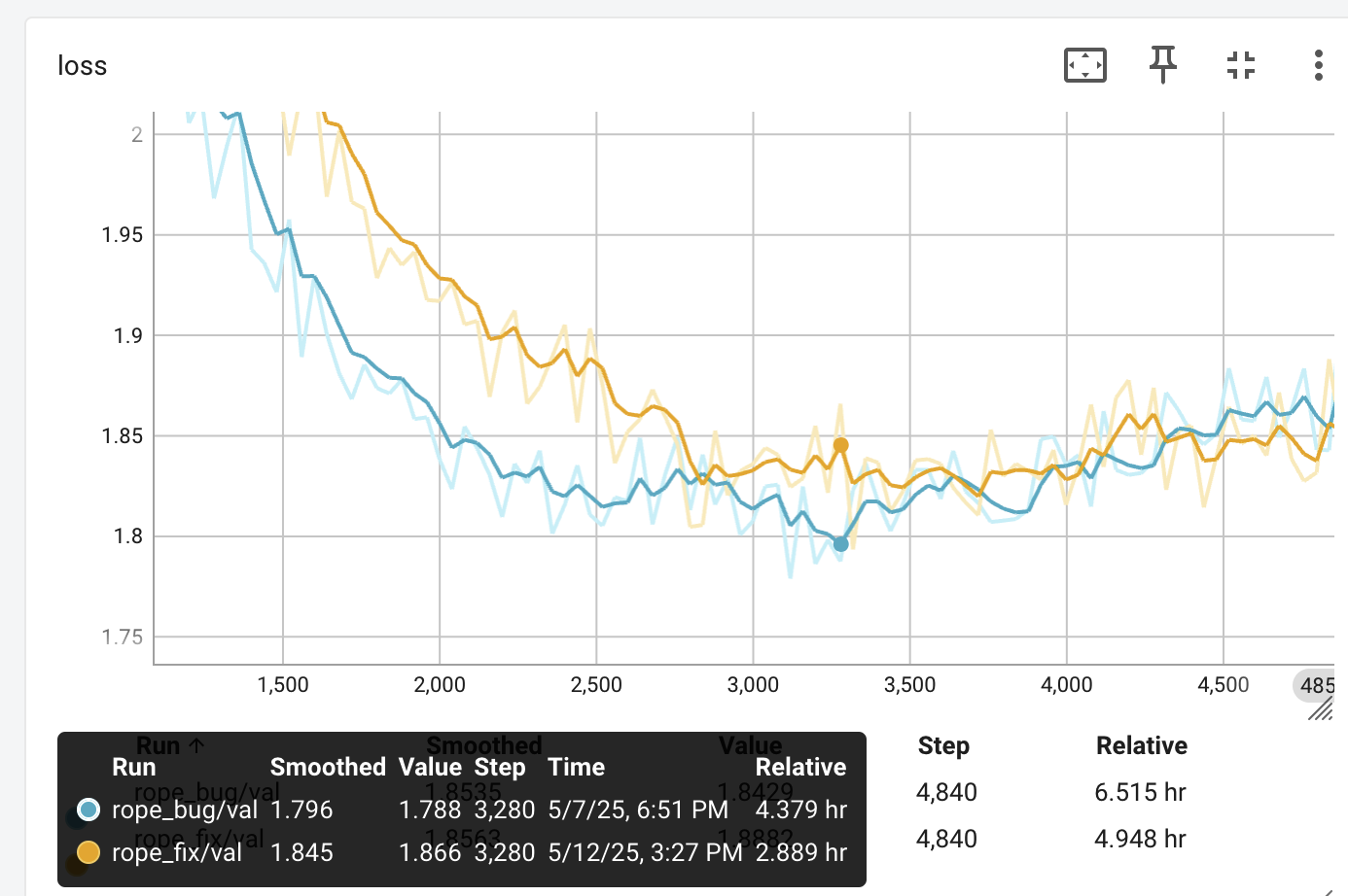
Classic overfitting:

A loss of 1.78 corresponds to a model that can’t decide between about six tokens for its output (e**1.78 ~ 6). Production LLMs, especially for structured coding - get to under two tokens.

Prompt Evaluations

The model was prompted every so often to complete

• A code snippet from the PyTorch repo
• A code snippet from this project

At epoch 8, step 3,120 - when the best validation loss is obtained, the prompt results were (using a temperature of 0.7)

Pytorch code:

prompt:

def lp_pool3d(
    input: Tensor,
    norm_type: Union[int, float],
    kernel_size: BroadcastingList3[int],
    stride: Optional[BroadcastingList3[int]] = None,
    ceil_mode: bool = False,
) -> Tensor:

completion:

class__ = "torch::executorch::Tensor"

    def __init__(self, input: Tensor) -> None:
        self.input =```

This Project Code:

prompt:

class MultiHeadAttnWithRoPE(nn.Module):
    def __init__(
        self, model_dim: int, num_heads: int, rope_encoder: RotationalPositionalEncoding
    ):
        super(MultiHeadAttnWithRoPE, self).__init__()
        assert model_dim % num_heads == 0, "model dim must be divisible by n_heads"
        self.model_dim = model_dim
        self.num_heads = num_heads
        self.rope_encoder = rope_encoder

        self.head_dim = model_dim // num_heads

        self.Q = nn.Linear(model_dim, model_dim)
        self.K = nn.Linear(model_dim, model_dim)
        self.V = nn.Linear(model_dim, model_dim)
        self.output_proj = nn.Linear(model_dim, model_dim)

    def forward(self, X):
        _, S, _ = X.size()
        q = self.rope_encoder(self.Q(X))  # B x S x D

(I gave it a long prompt!)

completion:

  </s> = X.T
  # Non-power Q and Q, float weight prepacked tensor
  # Yz, q, float eps, and float eps,

Hmm. I don’t know. That is nowhere near how I completed the function:

        k = self.rope_encoder(self.K(X))
        v = self.V(X)

        mask = torch.tril(torch.ones(S, S, device=X.device)).unsqueeze(0)  # [1, S, S]

        outputs = []
        for head in range(self.num_heads):
            d1 = head * self.head_dim
            d2 = d1 + self.head_dim
            qh = q[:, :, d1:d2]
            kh = k[:, :, d1:d2]
            vh = v[:, :, d1:d2]
            attn_vh = calc_attn(Q=qh, K=kh, V=vh, mask=mask)
            outputs.append(attn_vh)
        outputs = torch.cat(outputs, dim=-1)  # Concatenate on the last dimension
        return self.output_proj(outputs)  # Pass through the output linear layer

Did my transformer model do as well as Karpathy’s RNN?

I don’t think so. I have 3 times as many parameters, but he had 10 times more data. He predicted over next character, I over next token – using an off the shelf tokenizer on a small dataset.

Attention Plots

Ok, time for the fun stuff! We know Attention is at the heart of the Transformer! Let’s take a look at what the attention layers are actually doing! We’ll use the best model (on validation), modify the code to return the attention weights, and take a look!

Our architecture has four Transformer blocks, and each block contains four attention heads—giving us 16 independent attention mechanisms in total.

This branch: attnvis branch, hacks in returning attention weights when evaluating the model. This commit snapshots the code used for the plots below.

For every training batch, we compute a loss across the entire sequence length—from 0 up to 512 tokens in our case. That means for each example in the batch, at each position in the sequence, each of those 16 attention heads outputs a distinct set of attention weights.

One natural question is: how much are we attending to? To measure this, we compute the entropy of the attention weights (after softmax). High entropy indicates attention is spread evenly; low entropy that it is more focused or sparse.

For our maximum sequence length of 512, the maximum possible entropy (in bits) is 9 (since log₂(512) = 9). (I’ll use bits instead of nats for entropy units). So if we observe an entropy of, say, 8, that’s already significant—it suggests attention is concentrated over only half the sequence. To make this more interpretable, we exponentiate the entropy to get what we call the support: the effective number of elements being attended to.

For example, an entropy of 8 bits corresponds to a support of 2⁸ = 256 elements.

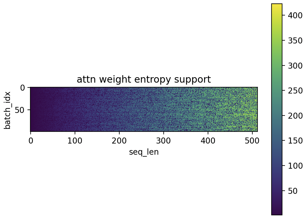
Batch of Attention Support

The first plot below shows a single batch—just to illustrate what support looks like. We can see that in some cases, attention is spread nearly across the entire sequence (support close to 400+), while in others it is much more focused.

We see that the masking is working - attention support never exceeds seq length in the batch.

Normalized Attention Support

In the previous plot, it’s hard to compare attention support across different sequence lengths. For example, when the sequence length is 1, the support is always 1—since the model can only attend to the first token when predicting the second.

To better visualize, we compute normalized support, dividing the support by the sequence length. Now, the maximum normalized support is 1.0, making values across different lengths more comparable.

We also include both training and validation data, using the same number of randomly selected batches from each.

This plot shows the distribution of normalized attention support across all 16 attention heads, along with overall mean. The spike at 1.0 likely corresponds to seq_len=1.

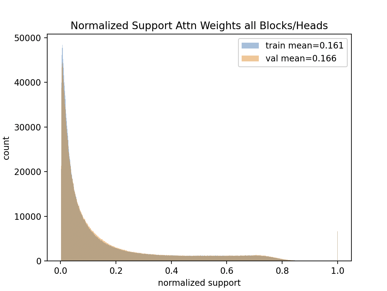
Note the overall means of 0.161 for train and 0.166 for validation - showing attention is a little more spread out for validation.

Normalized Attention Support vs Sequence Length

Normalized support depends on the sequence length. For example, an overall mean of 16% normalized support corresponds to just 1.6 tokens at sequence length 10, but 16 tokens at sequence length 100.

To better understand this, we visualize how normalized attention support varies with sequence length:

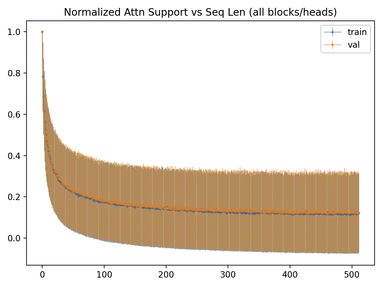
We again see how the support is a little higher for the validation split than train.

By Layer / Head

Finally, we take a look at how the attention support varies across different layers and heads. To make the results more comparable, we focus on a filtered range of sequence lengths. Each subplot in the 4×4 grid shows a histogram of attention support for a specific block/head, (block=layer) with both training and validation distributions overlaid.

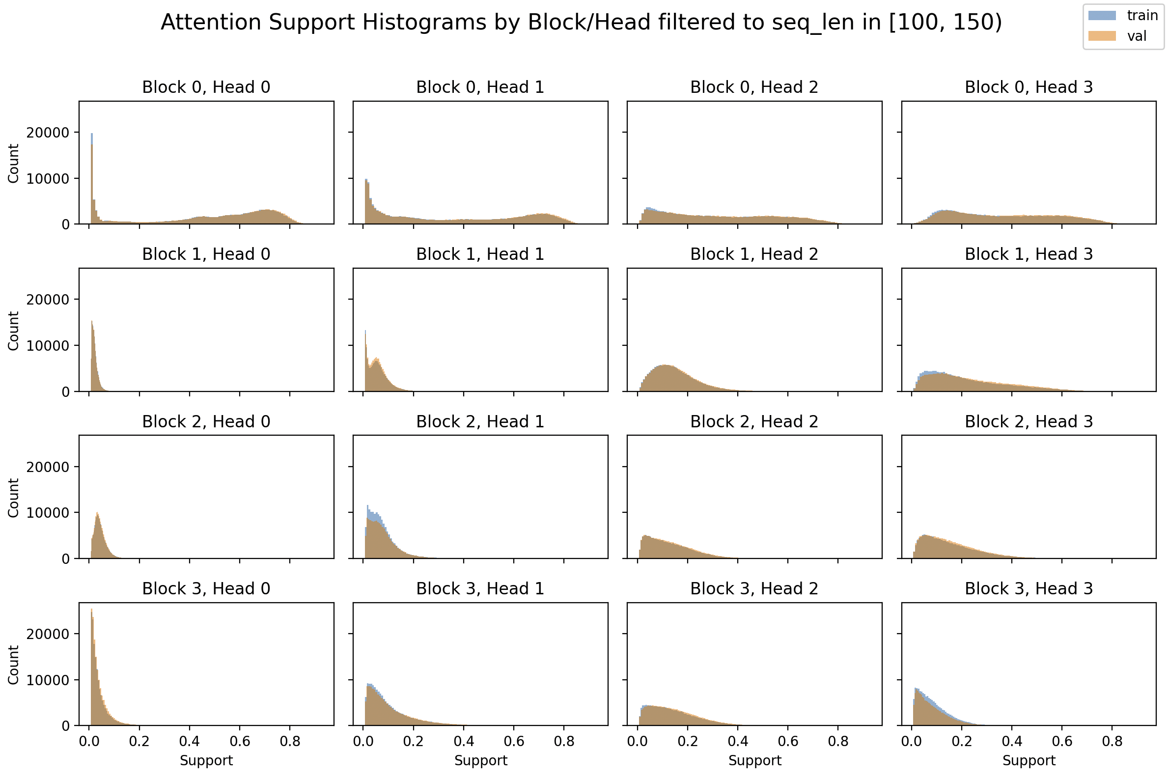
Observations: the first block (Block 0)—which directly processes the inputs—tends to have more broad attention.

In contrast, deeper layers seem to exhibit more focused attention, as seen in the narrower distributions in Block 2 and especially Block 3.

Another interesting observation is the apparent correlation among heads across layers. For instance, Head 0 in Blocks 1 through 3 seems consistently more concentrated near zero, unlike other heads.

However, this difference between the 0 heads and later heads seems funny. Read on …

Positional Encoding

I spent a lot of time thinking about, and implementing the positional encoding (settling on RoPE). The Hugging face blog You could have designed state of the art positional encoding is a great resource. It motivates why we need positional encoding in general, goes through additive positional encoding, and the arguments and value of rotational position encoding.

I got rotational positional encoding working, my model trained, things seemed good - but the layer / head plot got thinking more carefully about what I’d done, and led to the realization that I had a subtle bug!

Both additive and RoPE make use of vectors that roughly look like this:

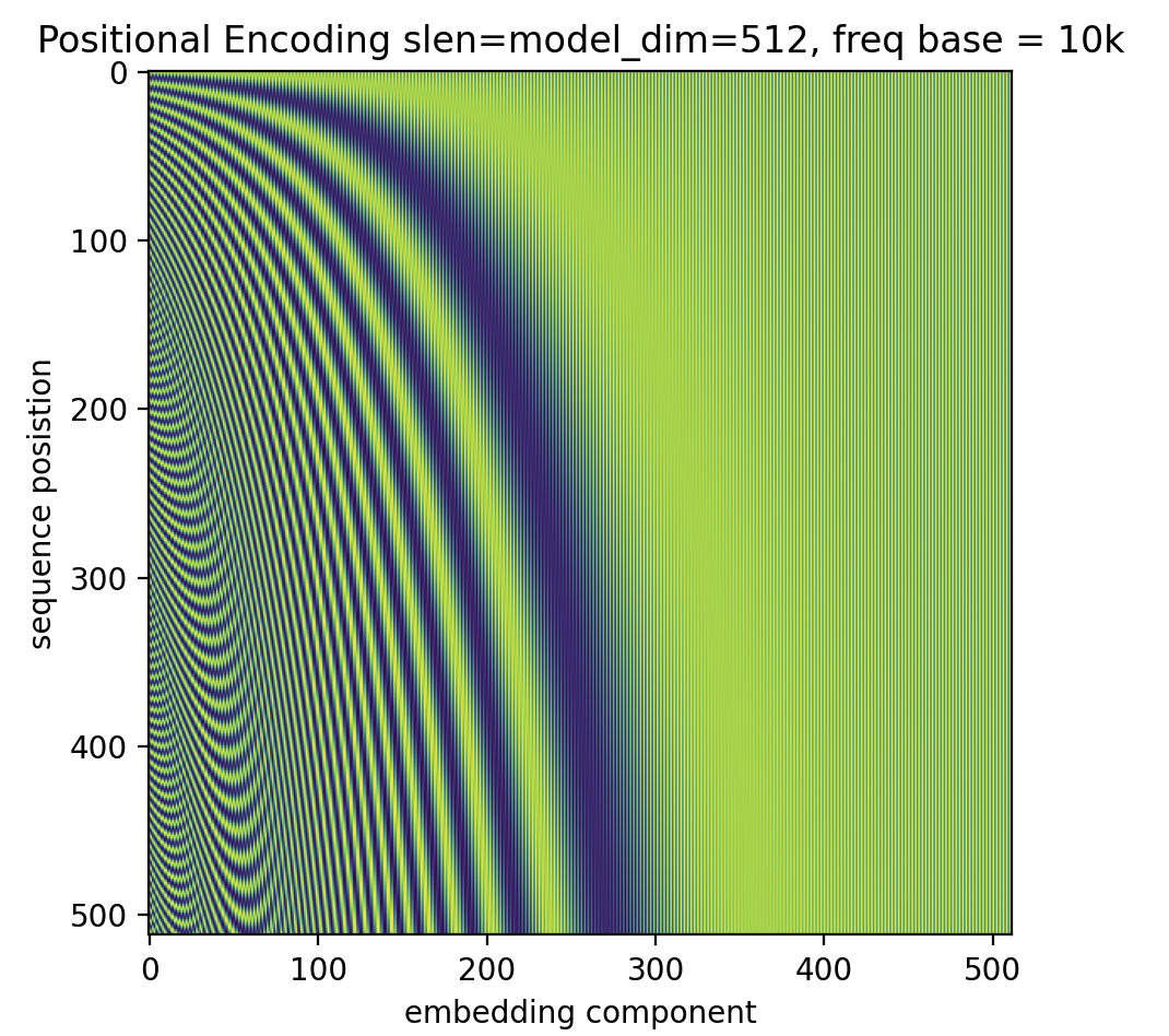
Additive positional encoding will add that to the inputs token vector embeddings that have been looked up from the original token ids.

Rotational, relative positional encoding will use them to rotate each two consecutive elements of an attention heads query and key components separately before computing the attention weights. In this way, the Q K^T computation will form relative differences in position, rather than adding fixed positions (see Hugging face post).

Implementation Issue

The way I implemented multi-headed attention + RoPE was to setup Q and K projection matrices

        self.Q = nn.Linear(model_dim, model_dim)
        self.K = nn.Linear(model_dim, model_dim)
        self.head_dim = model_dim // num_heads

and then produce q and k components for attention that first apply the RoPE encoding:

        q = self.rope_encoder(self.Q(X))  # B x S x D
        k = self.rope_encoder(self.K(X))

and then chunk them up for the 4 multiple attention heads:

        for head in range(self.num_heads):
            d1 = head * self.head_dim
            d2 = d1 + self.head_dim
            qh = q[:, :, d1:d2]
            kh = k[:, :, d1:d2]

but that means my first head is rotated by the fast frequencies:

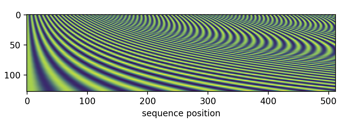
while my last is rotated by the slow frequencies:

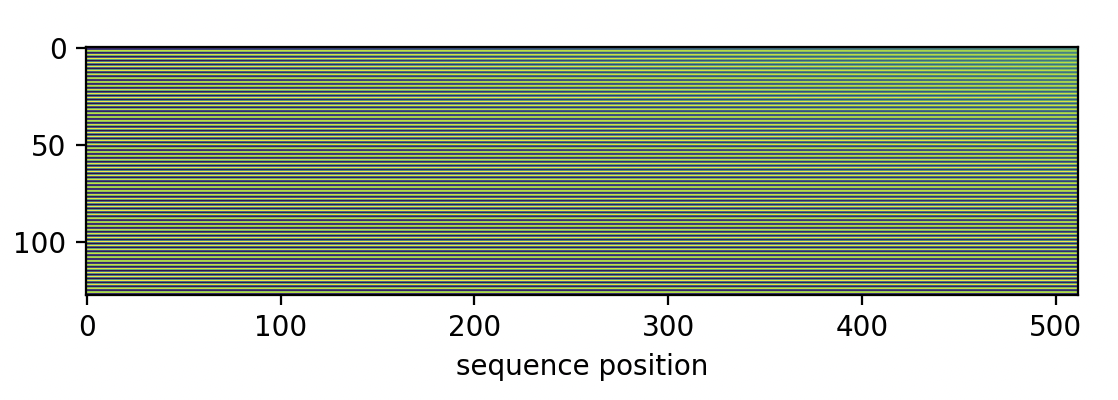
This was a subtle bug! Maybe you spotted it when reading the code in the prompting section? In any case, the same frequencies are supposed to be applied to all attention heads.

It is valuable to showcase how digging in, making plots, can help find subtle problems with machine learning implementations, but let’s see what kind of difference it makes to fix it.

RoPE Done Right?

The branch fix_rope applies RoPE with the same frequencies to each attention head. The frequencies are the 10,000 base introduced in Attention Is All You Need but now stretched to the head_dim of 112 rather than the model_dim of 448.

Loss

The training curves do not look very different - but one caveat is I did not fix the train/validation split - a different random 10% of the data comprises the validation for this run

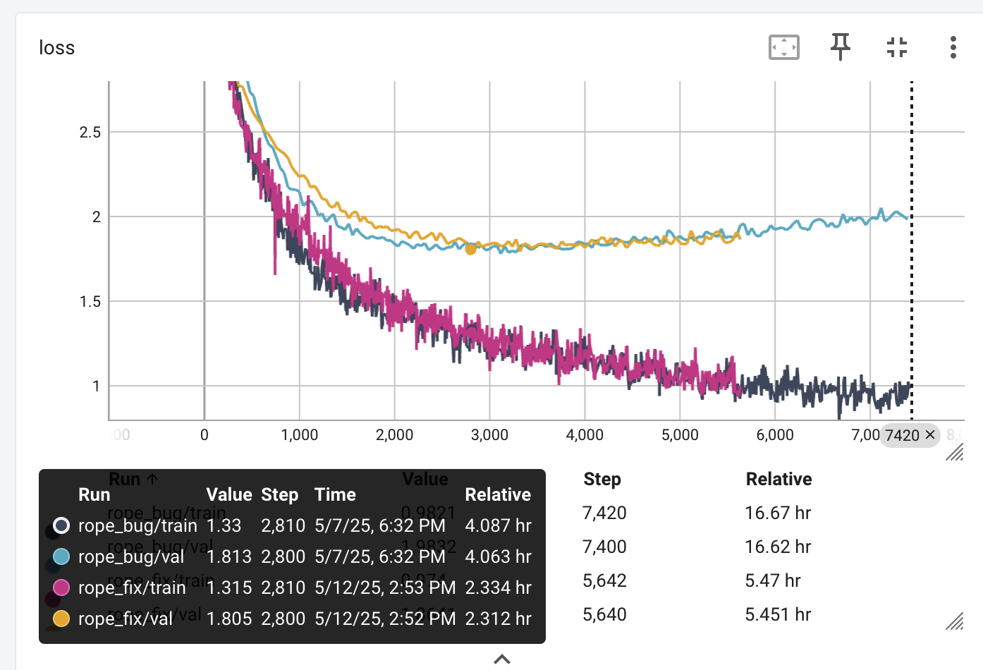
The validation loss is slightly better without the fix, on this new split of the data:

Prompt Responses

• pytorch code

   # Conv2d is not supported in the `maxpool3d`
  +-Exception = "latency"
    PT = 2 ** 2
    PT
  

• my code

    = self.Q  # B x V
       q = torch.randn(S, S, qsize, qsize, dtype=dtype)
       query
  

Below I’ll repeat the responses we saw with the bug:

• pytorch

   class__ = "torch::executorch::Tensor"
  
    def __init__(self, input: Tensor) -> None:
        self.input =
  

• mycode

  = X.T
  # Non-power Q and Q, float weight prepacked tensor
  # Yz, q, float eps, and float eps,

Not much difference?

RoPE Fix Attention Plots

Code for plots below is in the branch attn_fix_rope.

RoPE Fix Normalized Attention Support

The fix didn’t have much impact on the loss or prompts - maybe the bug was actually a happy accident worth exploring further, but now

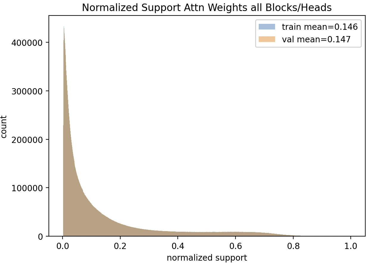
we are seeing some promising impact of the fix:

• the average normalized support has narrowed by 12.5% from .16 to .14
• The gap between train and validation has narrowed substantially.

RoPE Fix Block/Head Normalized Attention Support

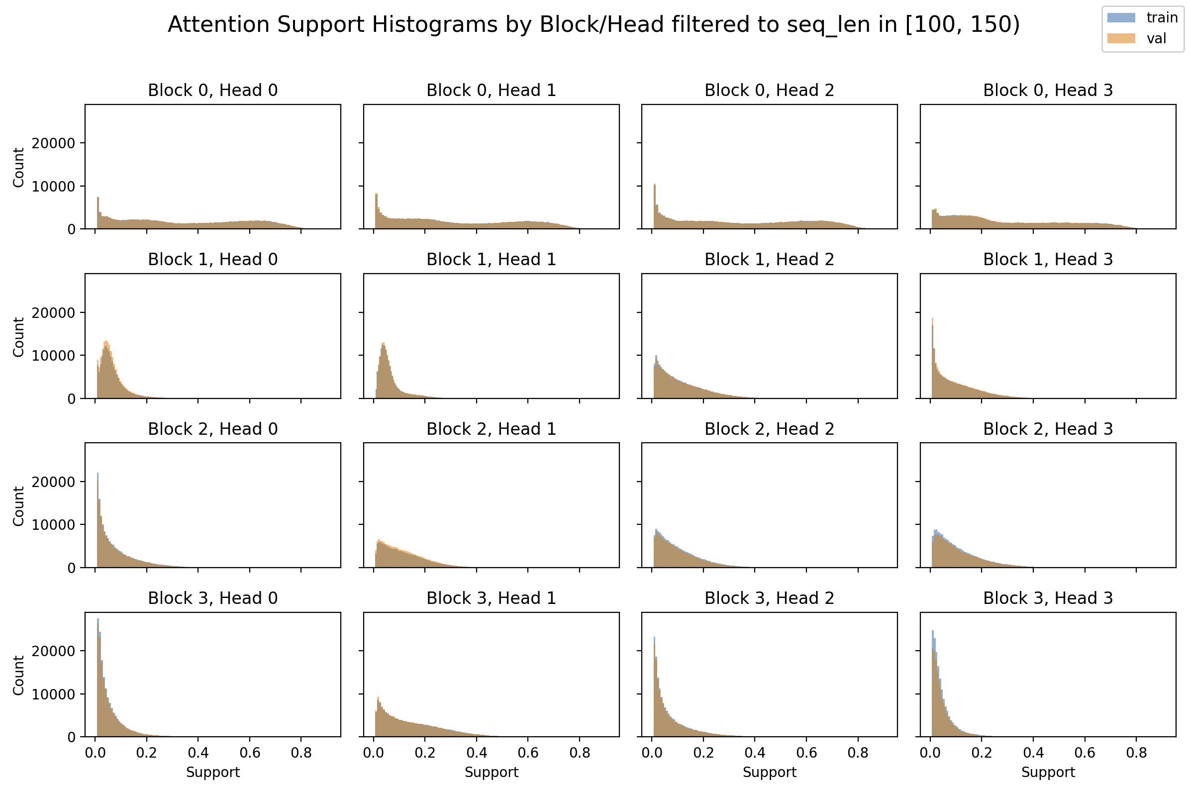
This looks better. I don’t see the big difference between head 0 and the rest that was present before the RoPE fix.

More Attention Plots

Emboldened by the value of visualizing attention support and diversity across heads, we now ask: what more can we observe to understand how the transformer works–and whether it’s working optimally?

Multi-Head Over Input?

How different are these heads? What are they attending to?

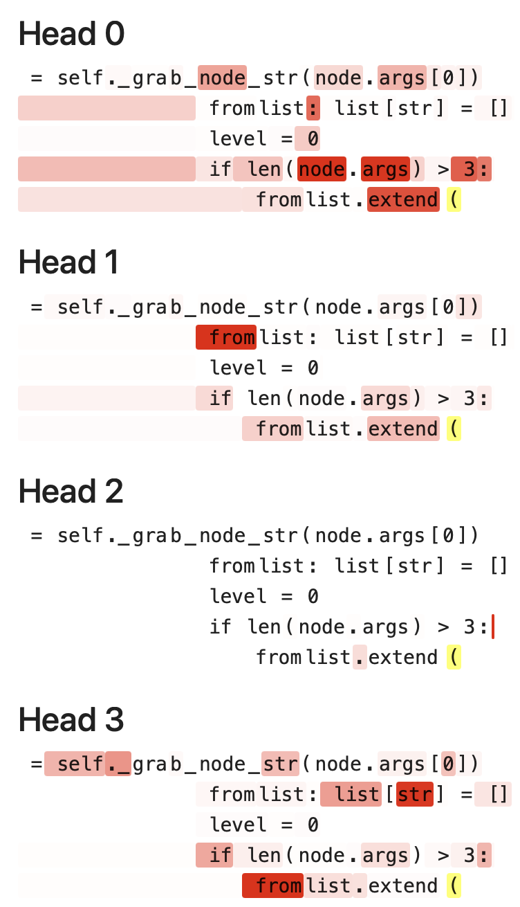
Continuing with the rope fixed model, here are the distributions of the four attention heads on the input layer, for a random training example of 50 tokens. Indeed. They are different :)

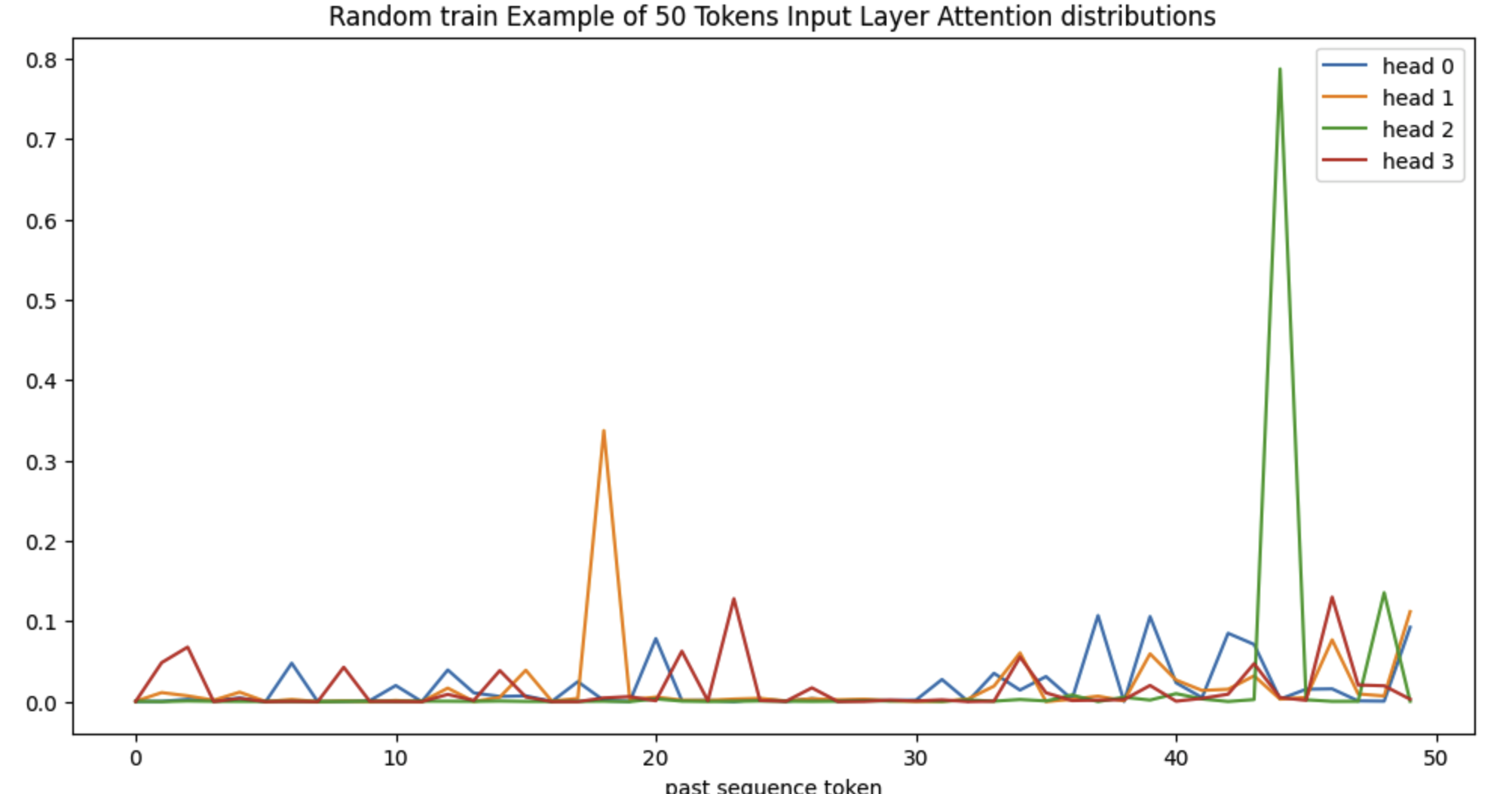
Below we’ve decoded the 50, and given a red background based on the attention probability. We scaled each head’s attention probability so that they are the same red color at their respective largest probabilities. The label to predict is in yellow:

Attention Diversity

How different do these heads get? Given two of the four heads in a block, we could compute the earth mover distance. Then we could average that over all the six pairs of the four heads. Maybe that would be an interesting metric to measure the richness of an input sequence for a layer? As there are six pairs per block, we could take the 24 earth mover distances that come from pairs of attention heads within a block, then take an average. That is, average these:

for headA in range(4):
   attnA = get_attention_distribution(headA)
   cdfA = cumsum(attnA)
   for headB in range(headA+1, 4):
      attnB = get_attention_distribution(headB)
      cdfB = cumsum(attnB)
      earth_mover_distance = sum(abs(cdfB - cdfA))

Would this somehow measure the complexity, or diversity of features that the whole model uses to predict on an input?

Let’s call that metric Attention Diversity. Restricting ourselves to sequences of length 50, where the maximum earth mover distance is 50, we get this histogram

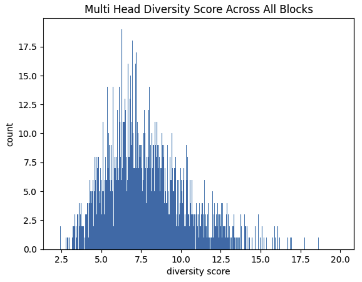
on a subset of the train split.

Simplest and Most Complex Inputs?

So what does the input look like for outliers of this metric? How might we interpret those inputs? The lowest attention diversity score is 2.2. And the highest is 20

Lowest Attn Diversity (score=2.2)

not getting gradient since the
            # output is unused in loss computation is supported. Specifically,
            # checks that the grads remain unchanged and are the same as local
            # training.
            inp = torch.randn(

and the token to predict is 10

Highest Attn Diversity (score=20)

        # prune the 4 smallest weights globally by L1 magnitude
        prune.global_unstructured(
            params_to_prune, pruning_method=prune.L1Unstructured, amount=4
        )

and the token to predict is seven white space characters.

I was hoping we might recognize a low score as simpler to complete and a high score as more complex - but I’m not seeing it :)

Compelling Ideas

To wrap up, here are a number of ideas that interest me for future exploration. I make no claim that any of these are new.

Vary Positional Encoding Across Heads

Accidentally using different encoding for the heads brings up the question - should the encoding be varied in some way? Would that allow the heads to learn a richer more diverse set of features?

Hard Attention?

I worked on a TabNet project in the past. A takeaway was hard attention is better than soft. The transformer uses soft attention - a softmax is applied to the query key multiplication Q * K^T to get the attention distribution. Even if the support is 16/512, the attention most likely attends to all 512 value components - but just with tiny weights for most. Would it help or hurt a transformer to use hard attention? I’d guess soft is better, seems you generally want to attend to everything in the past to some extent, and for creative outputs it probably helps. Practically, hard attention is much slower on GPUs so maybe it is a moot point.

Confidence Fine Tuning

For inference, we use a temperature parameter for LLM’s to control how creative/random its outputs will be. This only applies to the final logits over the next token. However, what about all the attention distributions over past tokens? Perhaps the model would achieve a better overall loss if we changed the temperature used in the softmax? Basically this equation

        /      Q * K^T     \
softmax |  --------------- |
        \  sqrt(model_dim) /

what if it was modified to be

        /            Q * K^T             \
softmax |  ----------------------------- |
        \  softplus(w) * sqrt(model_dim) /

where w is a new trainable parameter for fine tuning? With only one w for each attention head, this would be a very small set of parameters to train. Would be interesting to see how it compares to LORA. What if we let w vary with the sequence length? For each attention head, there could be one w for sequences of length 50-100, another for 101-200, etc.

Complexification

A desirable property for positional encoding is linearity:

positional_encoding(i) -  positional_encoding(j)  = positional_encoding(i-j) 

this is well explained with complex numbers through the phase, or θ in the e^{iθ} representation.

The arxiv paper that presented the RoFormer use complex numbers for the discussion.

Would be interesting to work over complex numbers for the transformer, in such a way (half baked idea coming) that the transformer block outputs track position through the phases.