Image Generative AI - DDPM
After digging into LLM’s with the Exploring the Transformer, Orthogonal Gradient Unlearning and Tokens and Unlearning posts, I’ve been eager to dig into image generation.
AI image generation took off with the paper Denoising Diffusion Probabilistic Models (DDPM) from 2020. DDPM produced higher quality images than the previous SOTA (state of the art) techniques such as GAN’s (Generative Adversarial Networks) and VAE’s (Variational Auto Encoders) by improving diffusion - a method introduced in 2015 in the paper Deep Unsupervised Learning using Nonequilibrium Thermodynamics.
This post covers the math of DDPM, and then switches into a research-style engineering log. I implemented DDPM from scratch with a simple model. I trained the model and sampled from it. Despite decent-looking training loss curves, the sampled images were wrong - they got darker and darker during the sampling. This led to an interesting investigation. I’ll go over developing metrics to get additional insights, and then running modified DDPM code from Hugging Face to get data points to compare to. We’ll end with a much deeper understanding of DDPM and many ideas to follow up on! We’ll wrap up with a literature search and summarize how many of these ideas have been followed up on in the last five years.
DDPM Math
The math in DDPM is built on VAE type posterior Bayesian analysis where one faces intractible integrals and makes approximations as with the ELBO (evidence lower bound). It breaks up image generation into a number of small steps - each that removes a little bit more noise from a starting image of Gaussian noise.
I have worked through much of the derivation of the DDPM loss in the notes below. These notes function as a companion to the paper, working through details rather than providing a complete story.
here is a PDF link to these notes as well.
There are many resources available to understand the math and DDPM – here are a few:
- Post by Lilian Weng
- Hugging Face annotated-diffusion easy to use code
- Notes from Stanford that include deriving the KL divergence of two Gaussians
Implementation
This section will go through the implementation and outcomes of the first run. For reference, the code is in this branch first_run of this repo. (see repo README.md about using/running the code.)
Data
For these experiments I resized the celebrity headshot dataset to 64 x 64. The original size is around 220 x 180. This was after wrestling with slow training. It let me load 200k images into memory (taking about 8GB RAM) to remove any data loading/preprocessing bottleneck.
However in hindsight, especially for the hardware I was using, better to start with smaller datasets. My hardware: 64GB RAM mac studio pro with M2 chip. I saw some impressive speedups with the Apple Silicon by using the pytorch mps device, but despite this, all my training runs were slow (taking days).
Small Dataset
The smallest dataset I saw for generative AI, is in the example code that accompanies the Deep Generative Modeling book by Jakub Tomczak. The dataset is load_digits from sklearn. For instance take a look at this VAE example notebook.
UNet
DDPM uses the UNet architecture from 2015 to learn how to denoise. Since my images were smaller, I tried a smaller simpler UNet - code link. It had no attention in the middle and was built just based on looking at the 2015 UNet paper. It ended up being quite small, too small I think - about 1/2 million parameters instead of 57 million in the next runs.
Incorporating t
The UNet takes both the image to denoise, and the timestep t. I took a simple approach to incorporating t into the model
- a sinusoidal embedding is made as in other work
- a simple nonlinear MLP learns something about it (the same kind of MLP you see in other work)
- however there is just one MLP - it is applied at the beginning of the forward pass
- different blocks that use the time as input learn linear projections resize it to the correct shape
Following DDPM
This first run followed the DDPM paper total number of timesteps to run the diffusion process: T=1000 and linear noise schedule with beta_1=1e-4 and beta_T=0.02. The noise schedule is how much Gaussian noise to add to x_{t-1} to get x_{t}, where beta_t is the variance of the added noise.
Outcomes
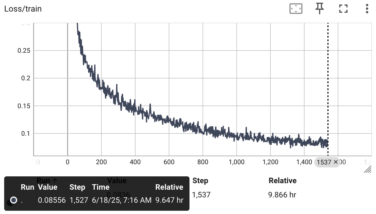
This first run had some interesting problems. Here is a plot of the training and validation loss curves - after 3 days:
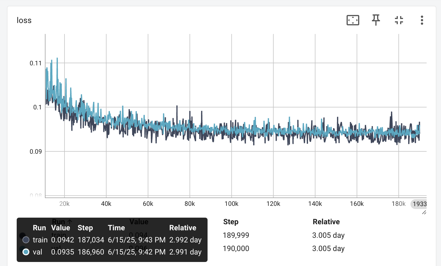
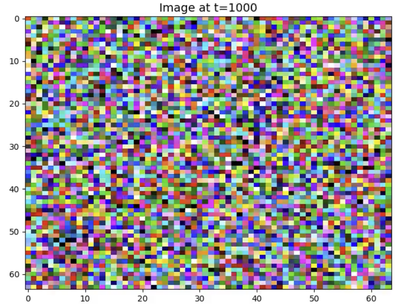
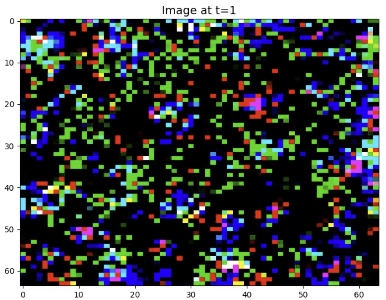
The first potential problem is slow convergence. However, if the images produced are good at this point, it is not a problem - but despite having learned something - the sampled images are bad. We start with pure Gaussian noise at t=1000 by sampling from N(0, I), but what we get from the reverse process at t=1 is:
|
|
The t=1 denoised image has a lot of black in it. Also some highly saturated RGB values.
Note that the preprocessed images have mapped the RGB values of [0, 255] to [-1, 1]. The noise we start out with at t=1000 is sampled from N(0, I). It can have values outside [-1, 1].
There is a lot of noise in DDPM. As you sample to make an image, you get new noise from N(0, I) for each timestep t. This noise is scaled and getting smaller as t gets smaller.
One can look at the histogram of values as we sample an image with this first run model.
The original sampled noise is mostly in [-1,1], but as we iterate from T=1000 down to t=0, we get more and more negative values (as well as more and positive):
Hypotheses
Bug
One hypothesis is a bug. DDPM provides the simple algorithm 1 for training and algorithm 2 for sampling. If there is a mismatch with these formulas - you could be removing more noise during sampling than you trained the model to represent.
Error Accumulation - Autoregressive Nature of Sampling vs Training
Another hypothesis is some kind of accumulation of numerical errors.
There are 1000 steps, in float32.
An interesting difference between training and sampling is that sampling has an auto-regressive property that training does not.
Sampling applies the model 1000 times to previous model output (and new noise) to get the next output - errors or model bias could accumulate.
Training on the other hand does not.
To train timestep t, we go straight from x0 and noise to get a training pair: x_{t-1} and x_{t}.
DDPM Training
In a little more detail, the model is learning the noise to remove at timestep t. Given x0, we can compute a x_t and x_{t-1} for training by getting two distinct Gaussians e_t and e_{t-1} from N(0|I) and taking an appropriate weighted sums (based on noise schedule, formulas for w_t and g_t in the DDPM paper and math notes above):
x_t = w_t * x0 + g_t e_t
x_{t-1} = w_{t-1} * x0 + g_{t-1} e_{t-1}
and then predict the difference, the model UNet(x_t, t) predicts e such that
x_{t} - e = x_{t-1}
Closer look
The findings above raise questions about the model’s performance at different timesteps. Two things to look at:
- Loss per t
- Model bias per t
Code reference for these metrics is the branch ddpmeval.
Loss per t
The loss is much worse at t=1 than t=1000
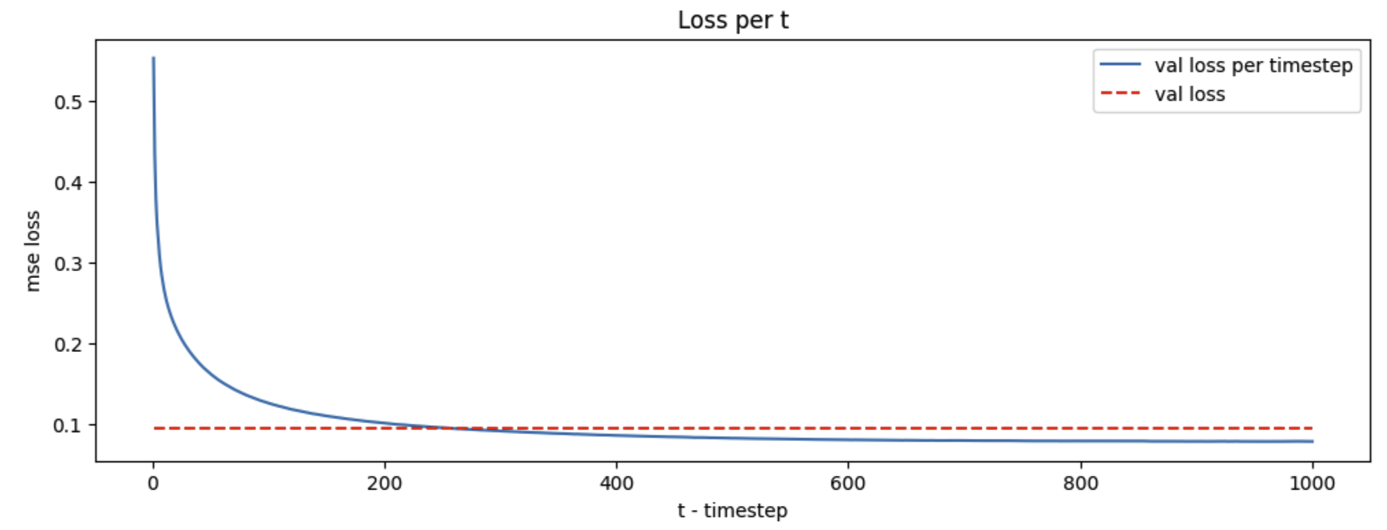
This looks bad - but we will see the same behavior for the Hugging Face code we run next - suggesting this is just how DDPM works, but why? Some thoughts:
- On the one hand, the scale of the model’s predictions aren’t changing over the timesteps
- it is always predicting noise
eps ~ N(0,I)- So shouldn’t the loss per
tbe about the same since it always predicts fromN(0, I)?
- So shouldn’t the loss per
- it is always predicting noise
- However much less noise is added at
t=1(variance = 1e-4) thant=T(variance=0.02) - In the limit, if we added no noise, we couldn’t predict anything - so the loss would be equivalent to what we’d get by making random predictions
- Therefore it makes sense the loss is worse for
t=1thant=T
- Therefore it makes sense the loss is worse for
- However it seems like it should be easier to remove that little bit of noise when we are close to a final picture, then a lot of noise when we are close to white noise?
Prediction Bias per t
The 2020 DDPM paper built on the 2015 diffusion paper in a few ways, and one is to reformulate the problem so that at every timestep t model predicts noise eps ~ N(0,I). Hence the predictions should have zero mean and a standard deviation of 1, for any t. This provides opportunity to diagnose training with a new metric - and it exposes a bias problem for the model:
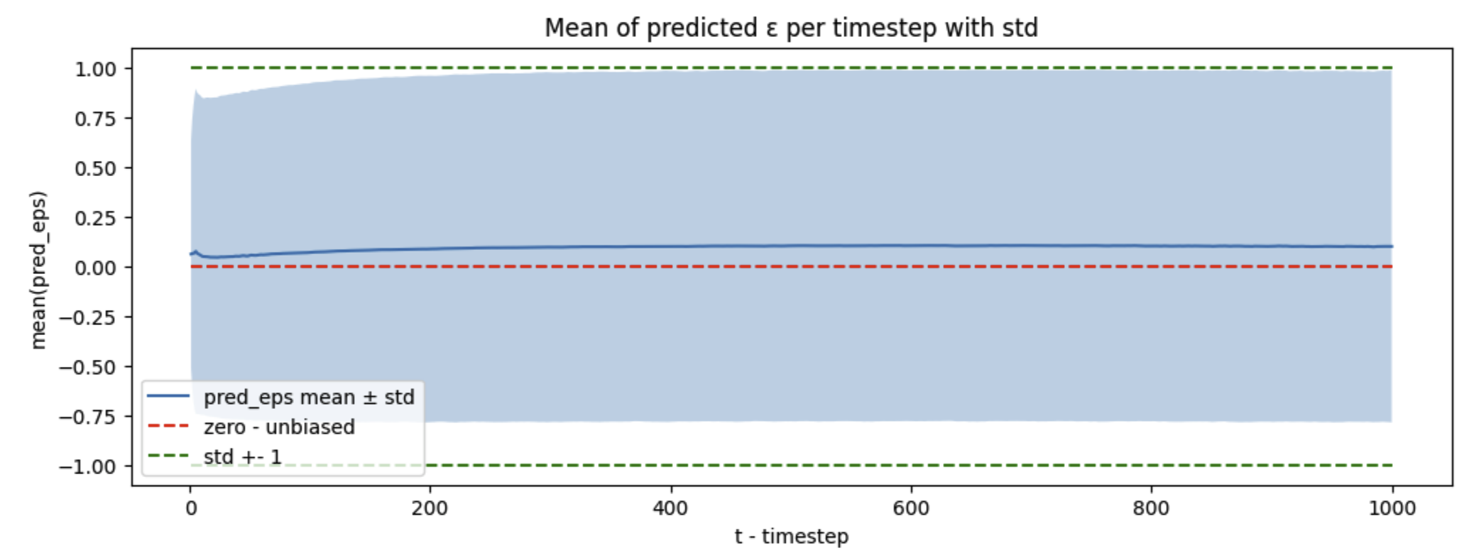
The mean prediction is not 0, it is positive (around 0.08).
An additional hypothesis for the problems we’re seeing is model capacity.
Hugging Face Code
The Hugging Face Annotated DDPM provides a colab that is easy to run - (also see this pytorch DDPM repo).
For reference I’m running it from this branch of my repo, using this modified notebook.
The UNet for this run has much more capacity:
- 50 million weights vs 1/2 million
- Visual attention layer
- Each UNet block has its own MLP to apply to the timestep embedding
- first run had one MLP shared among blocks
Other differences
- T=200 instead of 1000, use x5 less timesteps
- The original Hugging Face code applies random left to right flips of the data, but that is disabled for my memory cached dataset of celeba
After 10 hours of training, the loss is better than before, a testament to the higher model capacity
A sampled image has more structure, but we still don’t have celebrity faces. However from the loss curve we can see the model still has more it can learn

Interestingly, we see the same behavior with the loss per t, that is the loss is bad for low t

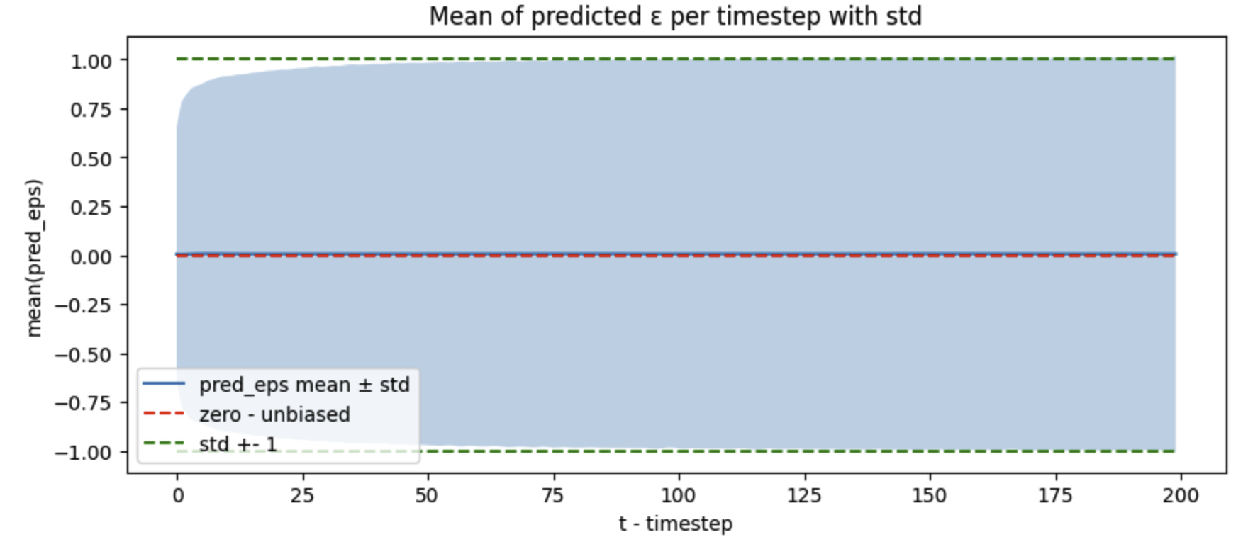
One thing that is fixed is the bias prediction - the mean of the predicted noise is now 0 and the std is 1:
Ideas
This analysis leads to a lot of ideas about improving the training.
Dropping Weights for Simple Algorithm?
We use the simplified algorithms in the DDPM paper - at the end of the math (see pdf notes above) we have a loss that is
L = L0 + L1 + L2 + ... + LT-1
where each of the Lt for t=1 ... T-1 is a MSE times a constant, that is
Lt = wt (ct eps_t - pred_eps_t(\theta))**2
and those constants wt are
betas = np.linspace(1e-4, .02, 1000, np.float32)
alphas = 1 - betas
sigmas = np.sqrt(betas)
alph_bars = np.cumprod(alphas)
wt = (betas**2)/(2*(sigmas**2)*alphas*(1-alph_bars))
that plot like
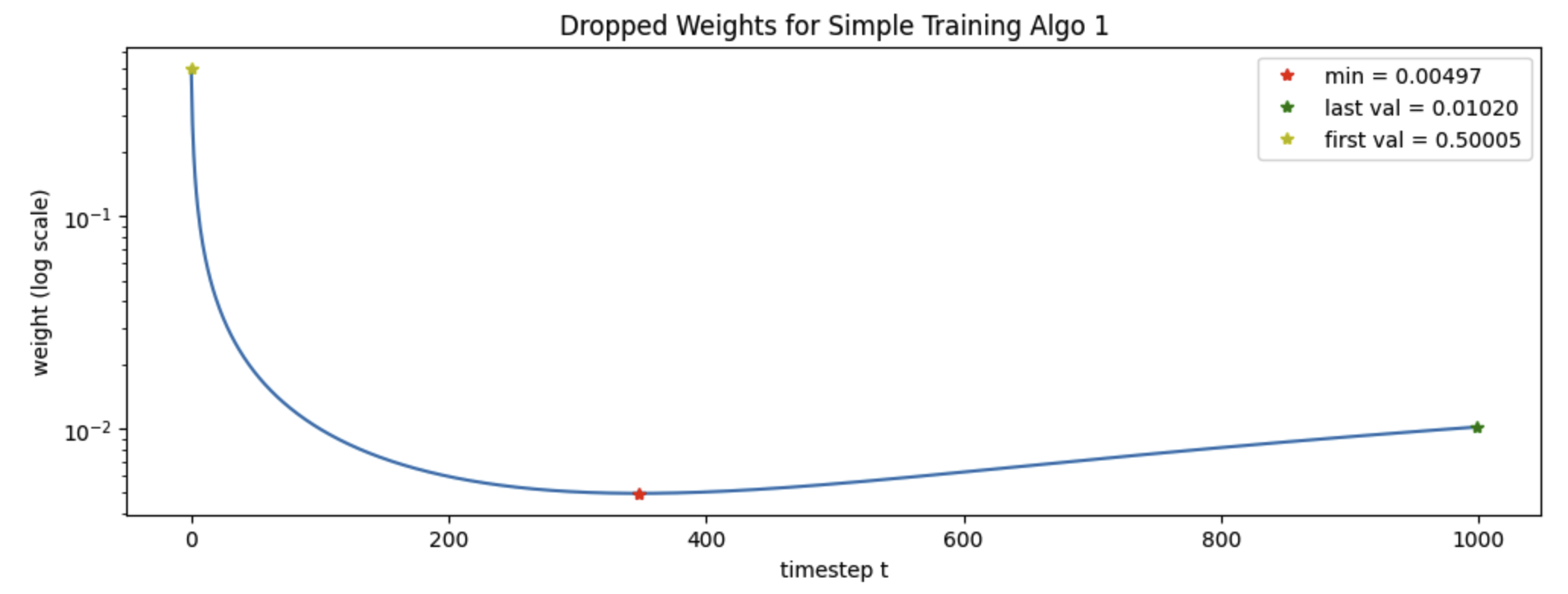
The simplified algorithm drops the wt from the loss that is used. The paper points out that later t are harder, so dropping these weights will help the model focus on the harder timesteps. The plot of the wt supports this, the wt clearly spike up for the early timesteps, however given the t-loss curve, I’m wondering if I’d like to keep the wt! Those big weights near t=1 might help the model train faster! However focusing on the loss too much can be a mistake - the highest quality images are not necessarily generated by the model achieving the lowest loss.
View Denoising Diffusion as a Multi-task Problem?
On the one hand, removing noise at t=1000 must be very similar to t=999, one model for both ‘tasks’ makes sense, but maybe removing noise at t=1 is very different?
It would be interesting to see what kind of loss we could get for a model trained only for the t=1 data.
Filters vs Unet?
Along the lines of the t=1 task vs the t=1000 task, for t=1, seems like image processing techniques like median filters would do a pretty good job – we only have a little bit of noise corrupting an image - we just want to smooth things out a bit, keep edges? Do we need visual attention, support that extends over the whole input for each output pixel?
For t=1000, where we are turning white noise into structured images - deep learning seems more critical. Experiments with multiple models for different stages of the diffusion process would be interesting. Perhaps a lighter, more image processing filter based model might be effective for earlier t values.
Boundary Values, Outliers
Sampling from N(0, I) will sometimes produce big values. At the end though, the RGB values of our preprocessed images live in [-1, 1] – with -1 being the most common value (especially for blue):
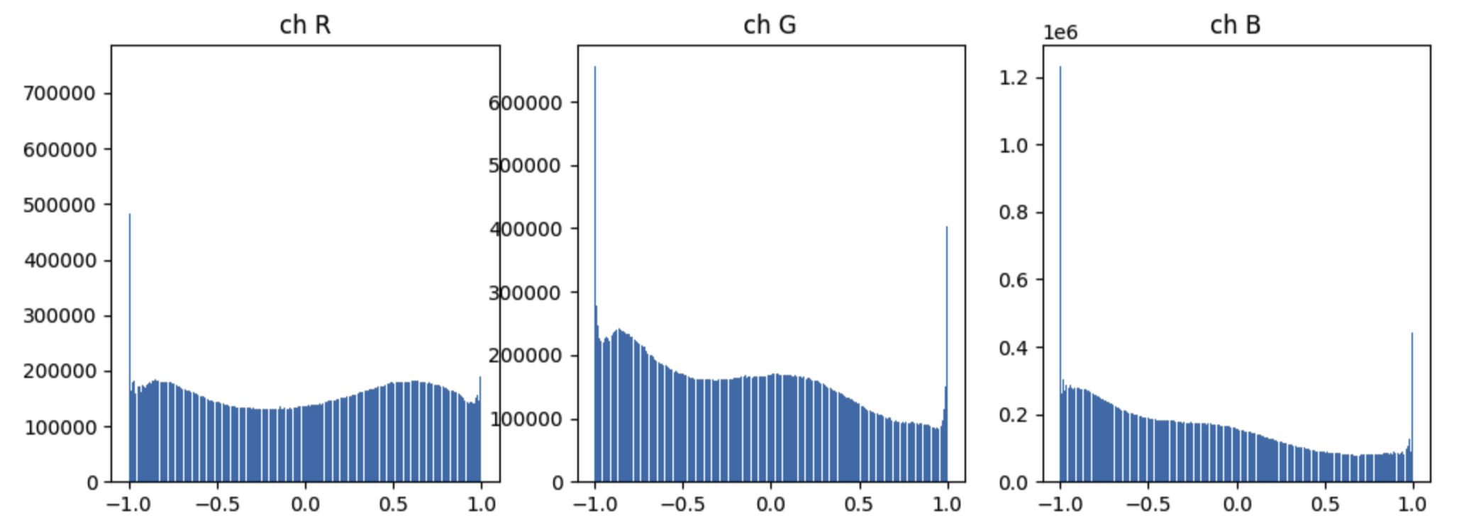
Given the slow training and dark saturation, I wonder if we should help the model predict these boundary values, and if outliers from sample noise create problems. For instance, if a low capacity model does pick up a bias - it seems those spikes at -1 would dominate.
Another aspect of the simple algorithm is it drops the L0 term. The L0 term is the loss that teaches the model how to do the final decoding - the DDPM paper provides a simple decoding that assigns a 0 probability to values outside [-1, 1].
Without the L0 term, I wonder if the model can become less ‘grounded’? more likely to predict large negative or positive values?
Possible experiments include:
- Adding the
L0loss - Using a Huber loss (as Hugging Face Annotated Diffusion does)
- Clip all noise used during training and sampling to
[-1, 1]
On the one hand, clipping is appealing, why not just keep everything in [-1,1]? That is what we want to end up with at t=0, why not start with it at t=1000 and along the way? This seems to be an easy way to eliminate outlier data that might throw the model off.
On the other hand, clipping reduces the entropy of the starting distribution – maybe the model needs more entropy to work with, to create new images from? There is also the question of the math, the beautiful math is derived using properties of normal random variables. We can (and should) make these kinds of easy changes to the final formulas to see if we get better image generation - but re-working the math using different distributions (if possible) could lead to better performance.
Hallucination and Timestep Stability
I would say my first run had bad hallucinations. There are good hallucinations where the model gets creative and comes up with new interesting things - but gradually darkening the image drifts too far from the target distribution. Bad hallucination.
It seems similar to how LLM’s can hallucinate. Training for LLM’s and DDPM is not auto regressive - you only predict the next token or noise to remove based on training data (as discussed above for DDPM). However I’d say there is an auto regressive nature to the sampling and inference, and hypothesize that it can be vulnerable to instability.
One approach to more stable sampling could come from numerical ODE solvers. There are a lot of techniques about making them stable. But perhaps this kind of stability development is more applicable to flow based models - perhaps that is why a recent SOTA model (the black forest labs FLUX.1 Kontext ) is flow based?
With a background in Geometric Mechanics, I am thinking about work like - Controlled Lagrangians and Stabilization of Discrete Mechanical Systems. Basically, if you write a numerical ODE solver for a mechanical system - you can leverage the fact that the total energy for the system will be constant over time. Developing an ODE solver that keeps the energy constant can improve numerical stability. However that won’t help if the system is inherently unstable - the classic problem in this field is the challenge of controlling an inverted pendulum. The method of Controlled Lagrangians derives the controller by first modifying the potential and kinetic energy of a mechanical system so that you
- Get stable dynamics
- Can split the equations of motion into
- the uncontrolled system
- and forces coming from a controller
the beauty is that the controller will be stable.
Training Multiple Timesteps
DDPM uniformly samples t and trains each stage independently. For a given x0 from the training data, we generate one input and output for the model to train on – the model will get input x_t and label x_{t-1}.
Could we train on a longer sequence? Using the model’s prediction for x_{t-1} to get to x_{t-2}? Sampling will use the model’s predictions - maybe they could be incorporated into training.
Why is Training Slow? A Lot of Entropy to Cover
With only 200k images, despite doing multiple epochs, my training runs had still not converged - but the model is not trained on just the 200k images - it is always trained on image + noise. We’ll never cover all the noise from N(0, I) over 3 x 64 x 64 = 12,288 dimensions - and it makes me wonder how many samples we need to train on to get good generalization from the model, vs how many might lead to overfitting, and memorizing the 200k training images.
The next milestone after DDPM was Latent Diffusion Models, carrying out the diffusion and denoising in the latent space, or bottleneck of a VAE trained on the images. Could an additional benefit of latent diffusion be how much less entropy the model must understand, as opposed to computational load of big images vs small?
How do these Ideas Resonate with the Field?
A lot of these ideas have been developed in the field.
Loss is typically higher at low-noise timesteps. Several works show that denoising small amounts of noise (e.g. at t=1) is harder for the model. Denoising Task Difficulty-Based Curriculum Learning from 2024 confirms that low-noise steps are empirically more difficult and slower to converge.
Noise schedule and loss weighting matter. The original DDPM used a linear noise schedule, but Improved DDPMs from 2021 showed that a cosine schedule distributes difficulty more evenly and improves performance. That same paper also proposed a hybrid loss that includes the L0 term (final reconstruction error), which can stabilize training and improve likelihood. More recently, Understanding Diffusion Objectives as ELBOs from 2023 analyzed how different timestep weightings affect optimization and gradient variance.
Sampling in DDPM is effectively autoregressive. While not autoregressive in the spatial sense, DDPM generation is sequential across time: each prediction depends on the last. This makes it vulnerable to error accumulation. Restart Sampling from 2023 shows that inserting occasional noisy steps during sampling can reduce this instability. Moving Average Sampling in Frequency from 2024 further stabilizes generation by averaging outputs across timesteps.
Flow-based models aim to improve stability. Recent models like Flow Matching for Generative Modeling from 2023 treat sampling as solving an ODE, which avoids the compounding errors seen in diffusion sampling. This idea likely underlies the new FLUX.1 Kontext from 2025, which emphasizes identity consistency and stable iterative edits.
Geometric and physics-inspired approaches are emerging. Hamiltonian Generative Flows from 2023 and Stable Autonomous Flow Matching from 2024 use ideas from Hamiltonian dynamics and Lyapunov stability to enforce stability and energy conservation during sampling.
Conclusion
Implementing DDPM from scratch and analyzing its training and sampling behavior led to several key insights:
- Sampling introduces autoregressive instability not present in training.
- Low-noise steps (e.g.,
t=1) are harder for the model to denoise effectively. - Model capacity significantly affects DDPM performance.
- Metrics like loss-per-timestep and prediction mean/std are valuable for diagnosing modeling issues.
Working through the math led to a second set of insights. DDPM starts from maximum entropy—pure N(0, I) noise—and gradually evolves toward a coherent image. As an artist, that feels like the reverse of how we create. I start from a blank slate—zero entropy—and add structure step by step: sketch, inking, color, shading, lighting.
It makes me wonder: can we build generative models that follow this more constructive process? I think modeling each artistic phase as a separate step would lead to powerful models giving users much more control over the artistic process.
The field has progressed a great deal since DDPM. With latent diffusion, autoregressive improvements, and physics-inspired methods like FLUX.1, I’m excited to explore what’s next!